P-value vs Effect Size
Overview
Usually data sets with massive sample sizes is a good thing. Well I would say it’s always a good thing provided you can hold it in memory. But sometimes large datasets can throw a wrench in your hypothesis testing.
If a stakeholder comes to me and wants to know if out if two samples are statistically different and their dataset has 500k observations, I know that whatever test I used would give me a significant result, telling me in essence that the samples were different. Well, that’s true, but how “different” are they? If I just give them a p-value of 3x10-20 and say, “yea they’re different” that doesn’t really help much (even if that is what they asked).
The Test
Let’s say this dataset is drawn from the same underlying distribtion. I can test that with the Two-Sample Kolmogorov-Smirnov (KS) Test. This is a non-parametric test looks at the cumulative distributions of the two samples.
The test statistic is the D-Statistic, or the maximum absolute difference between the two CDF’s.
The p-value answers the following question: What is the probability of observing a D-statistic as large or larger than the one I observed given the two samples are derived from the same distribution?
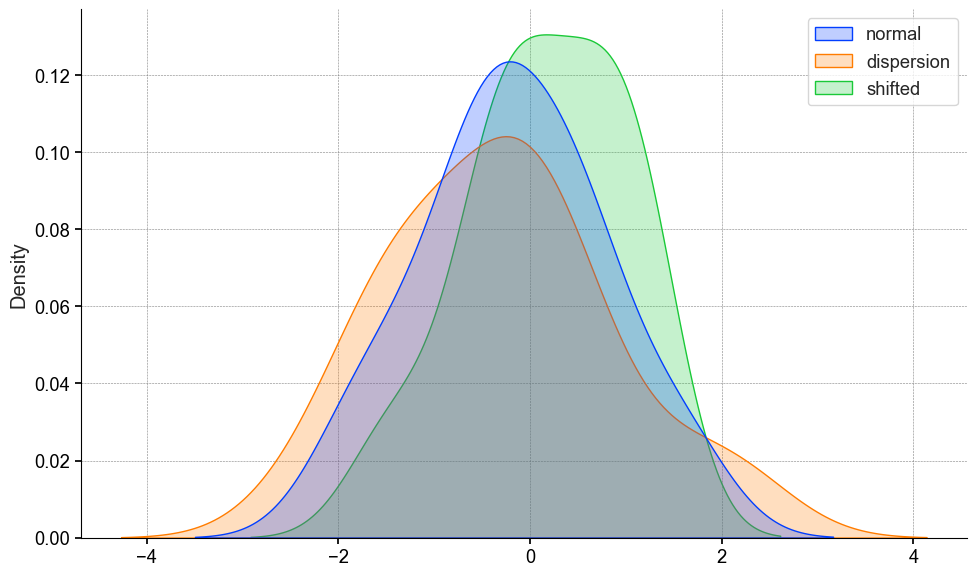
x = np.random.normal(loc=0, scale=1, size=20)
y = np.random.normal(loc=0, scale=1.2, size=20)
z = np.random.normal(loc=0.2, scale=1, size=20)
The KS test will compare the cdf’s to one another, and find the maximum absolute difference. Which is indicated by the blue dotted line.
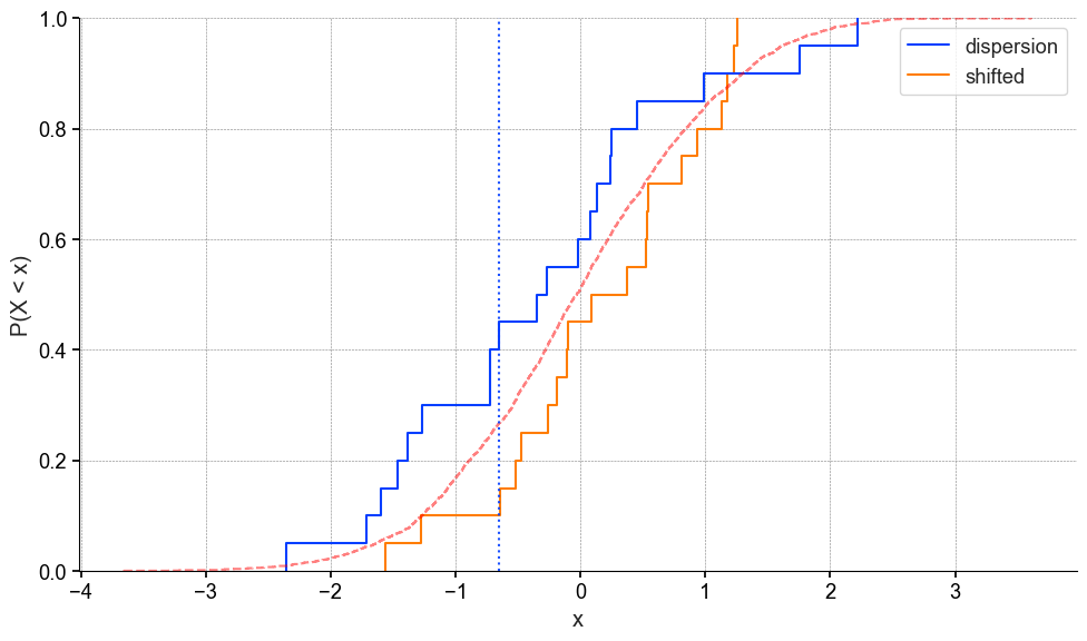
Now if you’re not familiar with empirical cumulative distribution plots, don’t worry they aren’t too common. The y-axis is interpreted as “the probability of observing a value equal to or less than x P(X < x)” and the x-axis is your variable of interest.
Decreasing P-value
As our sample size increases, the power of our statistical test increases, resulting in smaller differences being detected and smaller p-values being calculated.
# repeat for sample sizes 10 -> 1000
sample_sizes = range(10, 1000)

data = {n: [] for n in sample_sizes}

for n in sample_sizes:

    # data
    y = np.random.normal(loc=0, scale=1.2, size=n)
    z = np.random.normal(loc=0.2, scale=1, size=n)
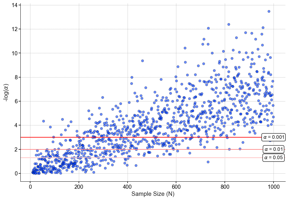
While I may anticipate this outcome, it will come as a shock (either good or bad) to the non-technical stakeholder waiting for my results. Now to be clear, the p-values to the right of the figure are not “incorrect” or “false positives”. As we can see in the code snippet, the data are indeed not the same, therefore as the sample size increases our test can pick up on these differences. That’s why it is important to look at sample size to put the results into perspective.
Effect Size
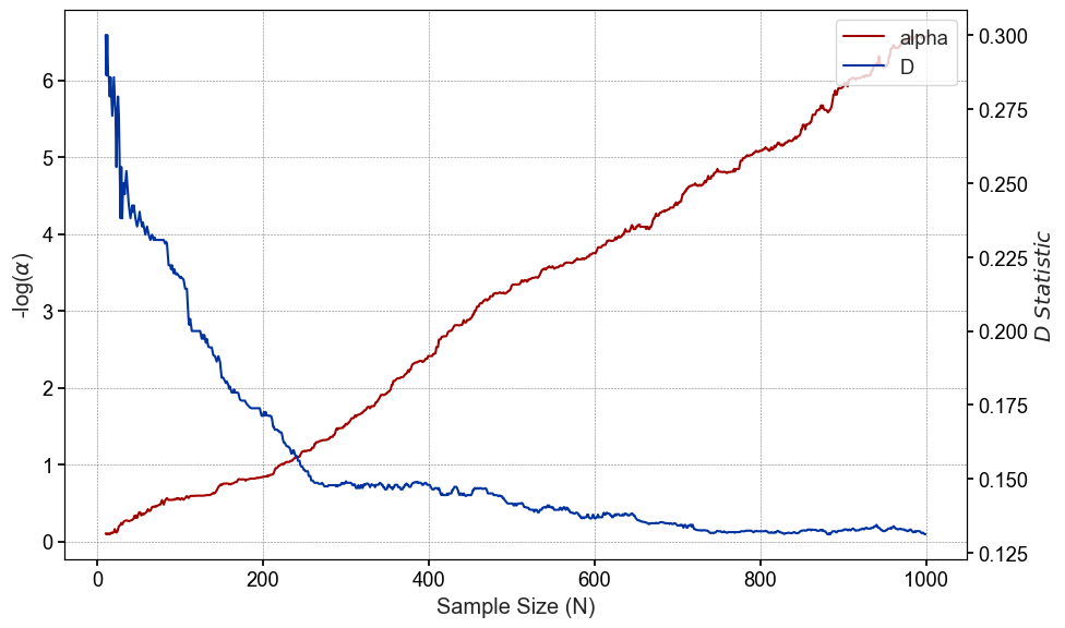
Unlike the p-value, our effect size does not increase or decrease linearly, but plateaus around n=200 and actually become less variable as the we approach sample sizes of n=1000
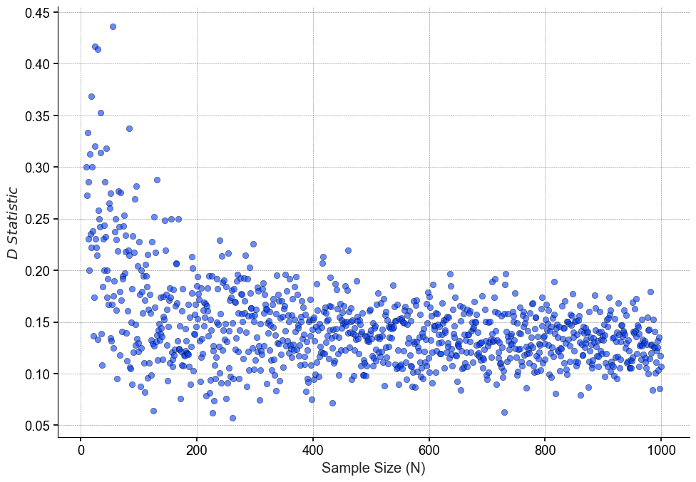
If we plot the rolling medians of both the p-value and D statistic, we can see more clearly how our the relationship between the two.
Wrapping up
For a lot of people, a p-value is sort of a yes or no metric. It’s different or not different. My intervention worked or it didn’t work. While a significant result in most classic studies is important because sample sizes are not infinite, it’s important to consider effect size to put significant results into perspective.
If you feel like this helped you out, feel free click the link below and support this post. Here’s my cat Vader for encouragement.
