Imputing College Tuition Prices- Log Tranformations
Imputing college tuition prices using sklearn
Overview

Today I want to experiment with log transforming the college scorecard dataset to see if this tranformation will mitigate the outliers that are positively skewing our data. If you haven’t seen our first round of imputation, feel free to check out the article here. In short, Random forest regression was the best imputation technique followed by bayesian ridge regression.
Log Transformation
As we saw in our first round of imputation, our data was positively skewed which was likely impacting the prediction power of many of these algorithms. A common way to mitigate this is by log transforming the variables which will hopefully normalize the distribution of the data and enhance the algorithms’ effectiveness, especially those assuming normality or linear relationships between features. A log transformation can also help reduce the impact that outliers will have on our data.
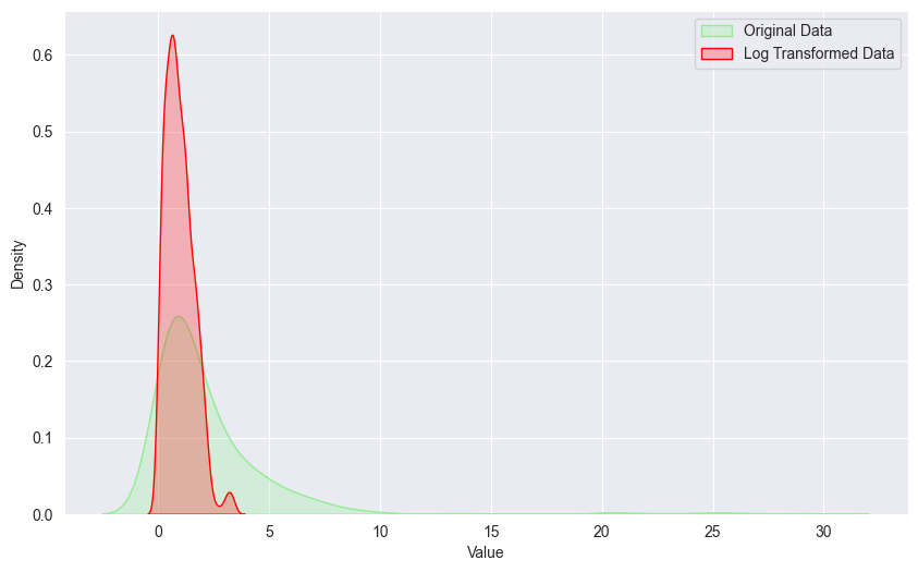
Because some of the values in our dataset are 0, and the log(0) = Undefined, we have to add a small constant to our dataset which will be 1.
# Log transform
test_df.iloc[:, 1:] += 1 # add small constant so no 0 values
test_df.iloc[:, 1:] = test_df.iloc[:, 1:].apply(np.log)
We won’t go through the training loop we wrote in the last article again.
Results
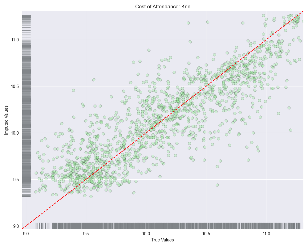
Looking at the scatterplots, it seems as though linear regression and bayesian ridge regression saw high amounts of variance at lower values potentially over-estimating values between 9.0-10.0. As we move to the right side of the plot these algorithms seem to then under-estimate the predicted values.
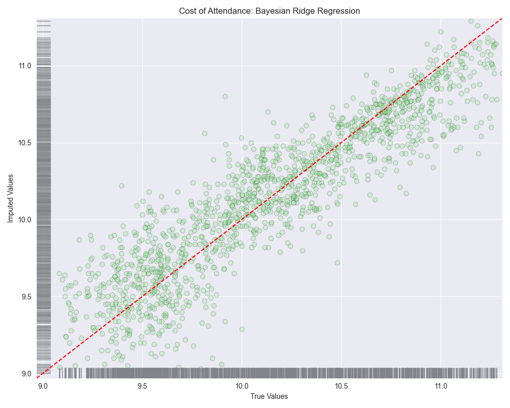
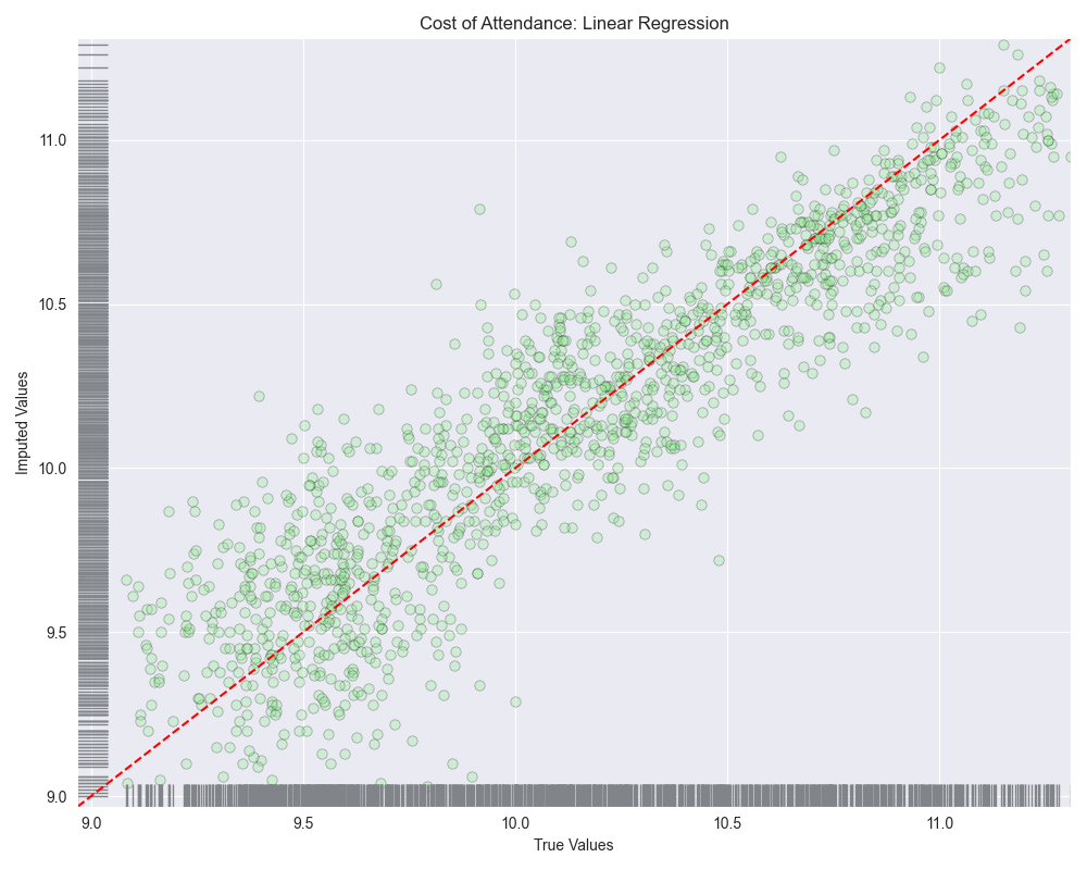
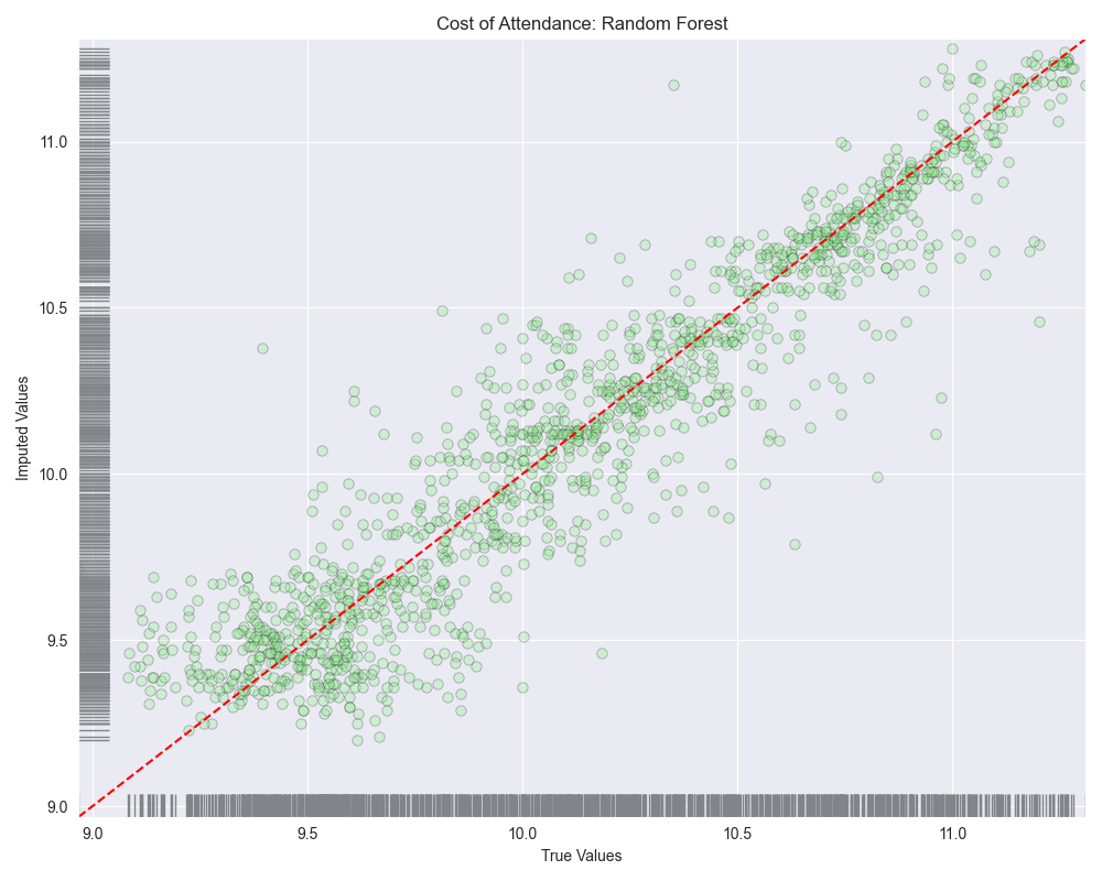
When we look at the residuals plots, we see that all of them exhibit some level of heteroscedasticity.
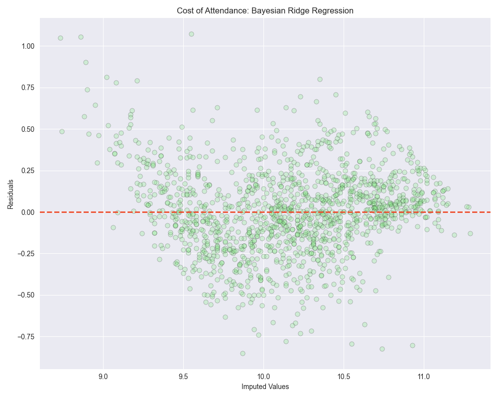
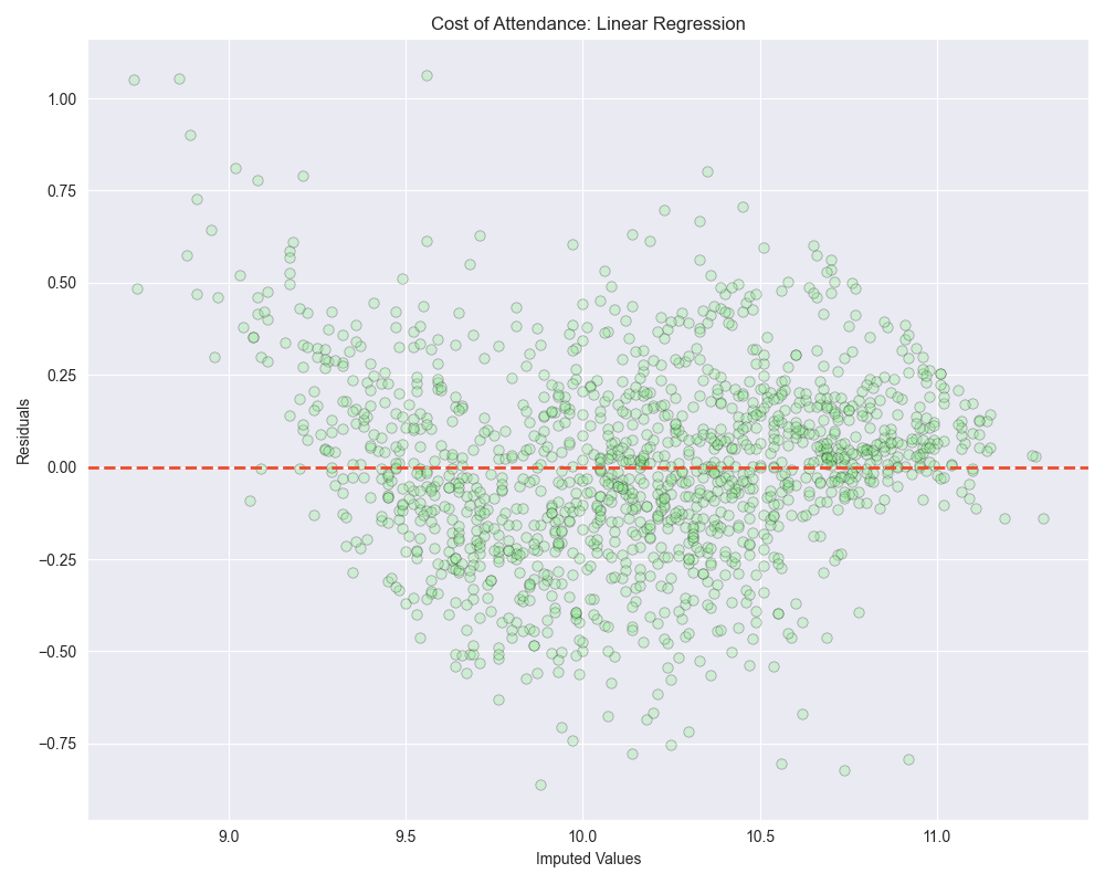
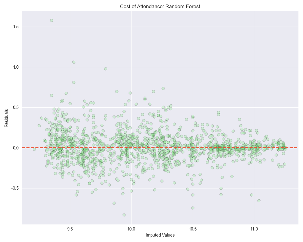
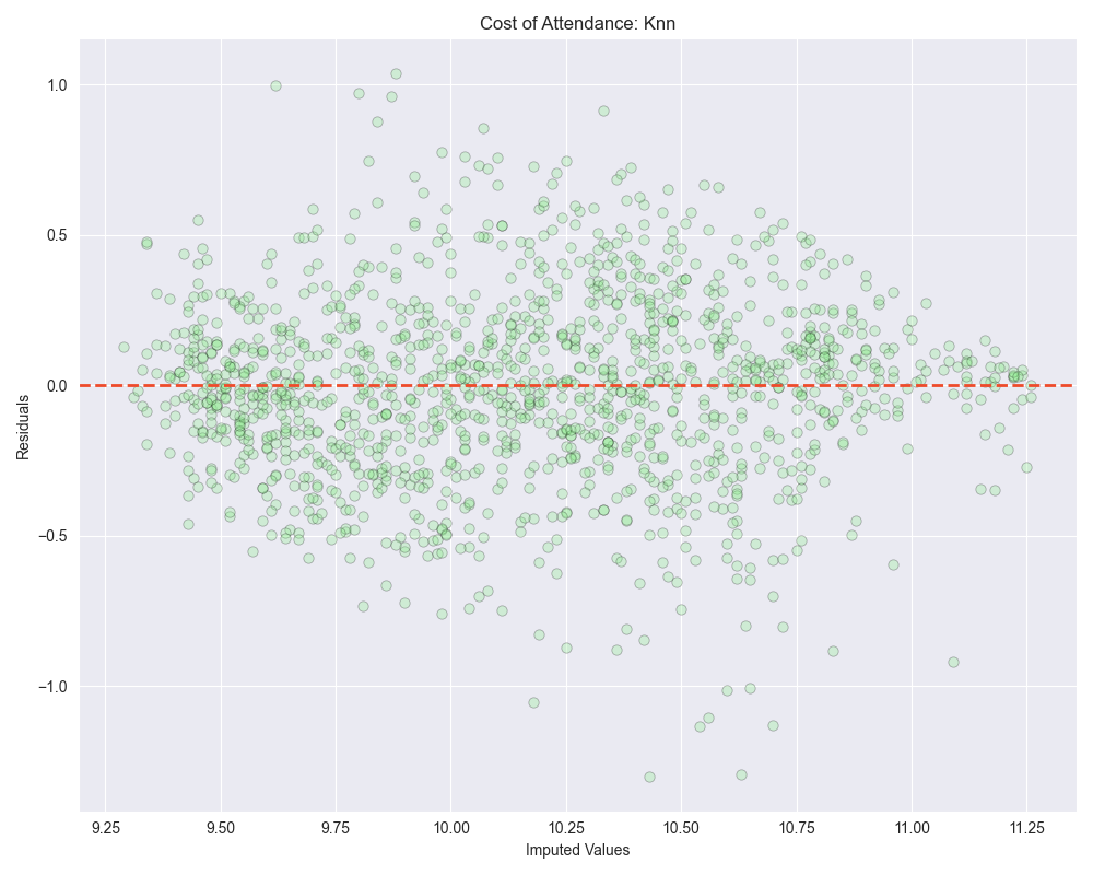
Heteroscedasticity is a situation where the variability (or “spread”) of the residuals (observed value - predicted value) in a regression model is not consistent across different levels of the independent variables.
In an ideal regression model, you want the residuals to be randomly scattered around the zero line, with no discernible pattern and a roughly constant spread throughout. This condition is known as “homoscedasticity,” which means “same variance.”
Our model has improved at handling outliers in our dataset from our last attempt, however there was a increase in MAE by 1.5%. Also, random forest regression seemed to do the best again-
Random Forest
- MAE: $3,481.87 > $3,535.72
- MSE: 30,602,315.13 > 29,873,710.69
- RMSE: $5,531.94 > $5,465.68
The runner up with this log transformed variable was actually linear regression, although bayesian ridge regression was very close behind. It’s also worth mentioning that linear regression did worse with the log transformed data than bayesian ridge regression did with the untransformed data:
- MAE: $4,292.5 > $5,345.28
- MSE: 37,296,221.96 > 58,008,514.88
- RMSE: $6,107.06 > $7,616.33
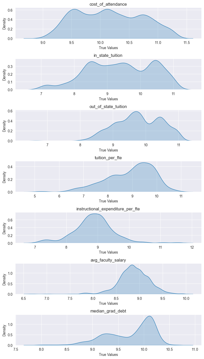
We can see that although the log transformation did reduce the outliers, it gave our features odd distributions, likely leading to the reduced performance of models other than random forest.
Conclusion
Overall, a log transformation enhanced our model’s robustness to outliers (well, only random forest really), it slightly affected its general prediction accuracy. Honestly though, the improvement to model performance was very minor, and at the cost of adding a slight bias to the model (+1 to entire dataset). Moving forward we will go back to the original dataset. Next up, One-Hot encoding! This will allow us to incorporate categorical variables more effectively into our models, potentially unlocking more insights and improving predictive performance.
If you feel like this helped you out, feel free click the link below and support this post. Here’s my cat Vader for encouragement.
