Intro

Today we are continuing our single-cell RNAseq series with an overview of how we go from raw reads contained in a fastq file to a nice data format called a count matrix.

If you need a brief introduction to fastq files go here where we went over the fastq file and wrote a script to parse this file type in Python.

If you haven’t seen the first article jump here where you can get an overview of 10x Genomics popular microfluidic-droplet scrna-seq assay.

If you want a brief intro to bioinformatic pipelines and even build one that calculates base quality scores with WDL, Python, and Docker check out this article here.

Let’s get started!

Overview of the processing pipeline

We’ve just ran our samples and got back some fastq files. How do we get to a count matrix?

If you recall, we have reads of sequences that were obtained from individual cells.

The reads have a cell barcode that tells us what cell the read came from.

The reads also have a unique identifier called a UMI which distinctly identifies each read.

Finally, recall that this was all done from the 3’ end of the read.

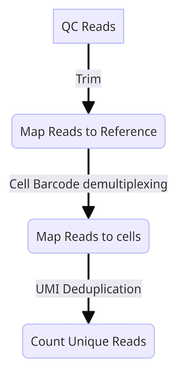
With this in mind, the general overview of the bioinformatic pipeline is as follows-

QC reads
Map reads to reference
Map reads to cells (cell barcode demultiplexing)
Count unique reads (UMI deduplication)

Step 1: QC reads

I abstracted some information away in the previous article for learning purposes, but now I’m going to layer in a few more points.

Along with the cell barcode (CB), the unique molecular identifier (UMI), and the DNA sequence itself, there is also something called a template switch oligo (TSO) sequence on the 5’ end and a poly-A tail on the 3’ end.

These are here because we actually reverse-transcribed our RNA transcripts to complimentary DNA before we sequenced the transcripts.

We reverse transcribed our RNA because cDNA is more stable that RNA.

The TSO and the PolyA sequences are a result of reverse transcription for reasons outside the scope of this article.

Because we have this TSO and PolyA tail in our fastq file we, we have to get rid of them. They’ll only make it more difficult to figure out the gene each read came from.

Step 2: Map reads to reference

After we get rid of the sequences that are not part of our DNA, we “map” the reads back to the genome.

This means we match the read back to the section of our genome from which it originated from.

To do this there are a few different tools called aligners that are often used like-

HISAT2
TopHat2
STAR

These aligners are pieces of software that- through algorithms and effeciently written code- align reads back to the genome.

Now, some of the reads will map to multiple places on the genome, these genes are referred to as “multi-mapped reads” these are removed.

Step 3: Map reads to cells

Before we try and figure out which cells these reads originated from and count our distinct UMI’s we have have to correct any sequencing errors.

As discussed in our previous article on fastq files, sequencers can make mistakes.

Sometimes they can mistakenly read an A as a C, or a C as T.

In light of this, we want to make sure that all of our barcodes are correctly read so we can assign the read to its cell of origin correctly.

To do this there are 2 major steps-

First, we compare all of of our cell barcodes to a list that 10x Genomics provides called a barcode whitelist. This list contains all the valid cell barcode sequences designed for the assay.
We compare the list of unique cell barcodes from our experiment to the barcode whitelist. We find all of the cell barcode sequences from our experiment that are not on the barcode whitelist differ by only a single nucleotide from any barcode in the whitelist.

If the 1 nucleotide that is different has a 0.975 posterior probability of being an incorrect base call, it is changed to match the cell barcode on the whitelist!

Note: Don’t worry too much about the “posterior” business for now, just assume that it means that there was a 97.5% chance that the sequencer made an incorrect base call.

Once we finish these steps we can assign each read to the cell it originated from.

Step 4: Count unique reads

After we have successfully mapped our reads to the cells and genes they originated from, all that’s left to do is count the UMI’s.

Just like we saw with the cell barcodes, a UMI can have a sequencing error as well.

To rectify this, a smiliar approach is taken. If two groups of reads have the same gene and cell barcode, but their UMI differs by 1 nucleotide, the group with less amplified reads and lower quality base scores is lumped in with the group with more reads.

Similarly, if two groups of reads have the same cell barcode and UMI but the genes they map to are different, the group with less reads is discarded.

In this scenario, if both groups have the same number of reads both groups are discarded.

Finally, we count all the distinct UMI’s in each cell and generate our count matrix!

The technical term is the unfiltered feature-barcode matrix.

It’s called an “unfiltered” feature-barcode matrix because it contains all detected transcripts, including those that may later be removed for being likely artifacts or noise.

Outro

And that’s it! In the next article we will dive into downstream analyses.

Here are some great resources that go into these steps in more detail if your curious.

10x Genomics algorithms overview Sanger Institute Broad course 10x Genomics barcode sequencing correction whitepaper

I hope you found this useful and see you in the next one!