Imputing College Tuition Prices
Imputing college tuition prices using sklearn
Overview

College is expensive, and only getting more expensive year after year. Whether the investment is worthwhile from a financial standpoint is a discussion for another day. What I do want to address is the issue of price transparency in higher education, which is problematic at best. The reason why price transparency isn’t the best is a question I don’t have the answer to.
College Scorecard
If you haven’t heard of the college scorecard, you aren’t alone. The College Scorecard dataset is a comprehensive and publicly available dataset provided by the U.S. Department of Education. It contains information about various colleges and universities in the United States and is designed to help students and their families make informed decisions about higher education. Now in all fairness, the U.S. Department of Education has made these data more accessible via a web tool at https://collegescorecard.ed.gov/ where you can query the data more effectively.
Some of the data available in this dataset are as follows:
- Admission statistics
- Graduation rates
- Median earnings of graduates
- Student demographics
- Average costs and financial aid information
- Institutional characteristics
Data Imputation
Although this dataset is large and very comprehensive, there is a lot of missing data. Ideally, all universities would share the cost of attendance, but that isn’t always the case. In this project we are going to try to impute missing values via 4 different methods:
Linear Regression
Linear regression imputation is fairly straight forward. It involves predicting missing values by fitting a linear model to the observed data. This model estimates the relationship between the variable with missing values and other relevant variables in the dataset.
Bayesian Ridge Regression
Bayesian ridge regression is similar to linear regression imputation. This technique incorporates a Bayesian approach and considers the uncertainty in the model parameters by assigning prior distributions. This approach is hopefully going to be particularly useful with dealing with the multicollinearity we see in our dataset. This model estimates the posterior distribution of the missing values, providing a range of plausible imputed values along with their probabilities. For the sake of simplicity we won’t get into the probability of each imputed value and just take the value with the highest probability.
Random Forest Regression
Random forest regression uses an ensemble of decision trees to predict the missing values. Random forest models are robust and can handle non-linear relationships, interactions between variables, and multicolinearity among variables as well. Multiple decision trees are trained on the observed data, and the missing values are predicted by aggregating the predictions from individual trees.
K Nearest Neighbor Regression
KNN imputation involves predicting missing values by considering the values of their k-nearest neighbors in the observed data. It’s based on the idea that similar instances have similar values for the variable of interest. For each missing value, the algorithm identifies the k-nearest neighbors in the observed data and averages their values to impute the missing value. I am going to leave k at 5 for this demonstration, but I would imagine there is a hyper-parameter tuning technique that we can explore after this initial dive.
About The Data
If you would like to see the results of the analysis, scroll down to the “First Try” section. Below I am going to describe each field in the college scorecard that I will be using for this analysis:
- COSTT4_A The average annual total cost of attendance, including tuition and fees, books and supplies, and living expenses for all full-time, first-time, degree/certificate-seeking undergraduates who receive Title IV aid. For academic-year institutions, average cost of attendance represents an average of all programs and includes only full-time, first-time, degree/certificate-seeking undergraduates who first enrolled in the fall term. For non-academic-year institutions (program or continuous enrollment), average cost of attendance represents the program with the largest enrollment at the institution, and it includes full-time, first-time, degree/certificate-seeking undergraduates who first enrolled at any time during the academic year. For programs less than 1 year in length, this represents the cost for the full program.
- CONTROL Control is the ownership of the institution with 1=Public, 2=Private non profit, 3=Private for profit.
- GRAD_DEBT_MDN The median debt for students who have completed/graduated.
- ** TUITIONFEE_IN** In state tuition.
- TUITIONFEE_OUT Out of state tuition
- TUITFTE Net tuition revenue (tuition revenue minus discounts and allowances) divided by the number of FTE students (undergraduates and graduate students).
- INEXPFTE Instructional expenditures divided by the number of FTE students (undergraduates and graduate students).
- AVGFACSAL Average faculty salary per month, calculated from the IPEDS Human Resources component. This metric is calculated as the total salary outlays divided by the number of months worked for all full-time nonmedical instructional staff. Prior to the 2011-12 academic year, when months worked were reported in groups, the value for 9-10 months is estimated as 9.5 months and the value for 11-12 months is estimated as 11.5 months. Values prior to the 2003-04 academic year are limited to degree-granting institutions for consistency with values in subsequent academic years.
First Try
As I mentioned earlier, this dataset has null values of the following proportion in each column:
| Column | Null Proportion |
|---|---|
| CONTROL | 0.0 |
| REGION | 0.0 |
| GRAD_DEBT_MDN | 2.4 |
| COSTT4_A | 49.5 |
| TUITIONFEE_IN | 42.1 |
| TUITIONFEE_OUT | 42.1 |
| TUITFTE | 7.9 |
| INEXPFTE | 7.9 |
| AVGFACSAL | 40.3 |
| LOCALE | 7.5 |
Our approach is going to be as follows:
- Remove all nulls from the dataset.
- Randomly assign nulls to the dataset that is proportional to the actual nulls in the original dataset. We are going to do this so that when we impute the data, we can get some error metrics and see how close we were.
- Impute values.
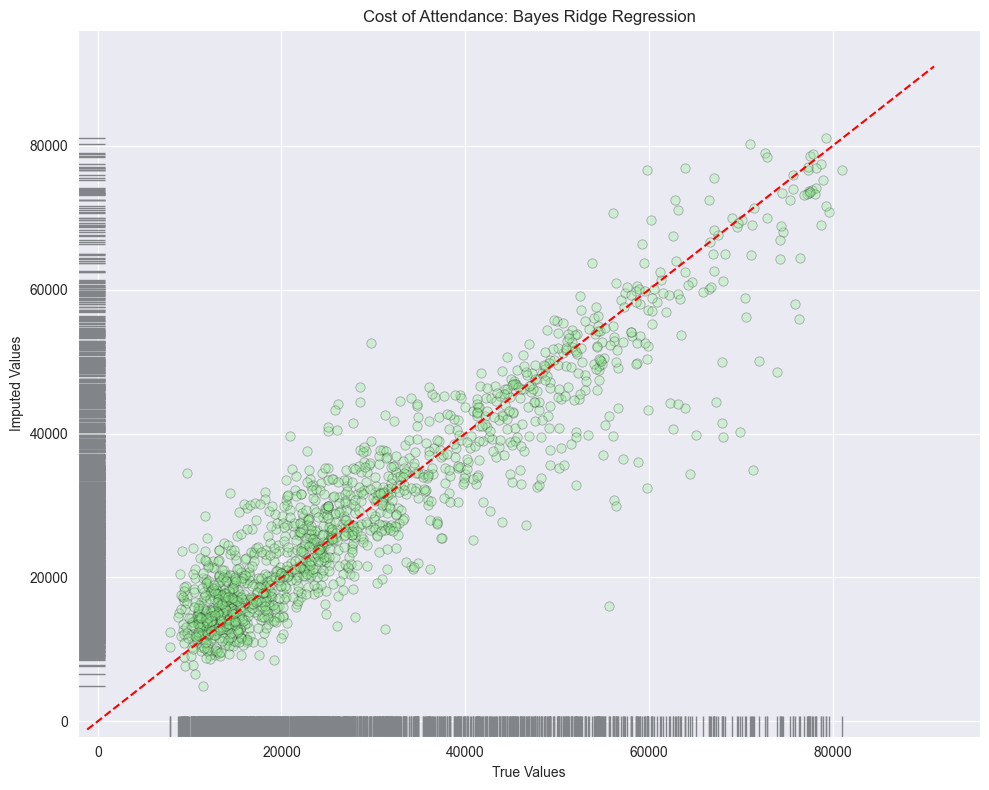
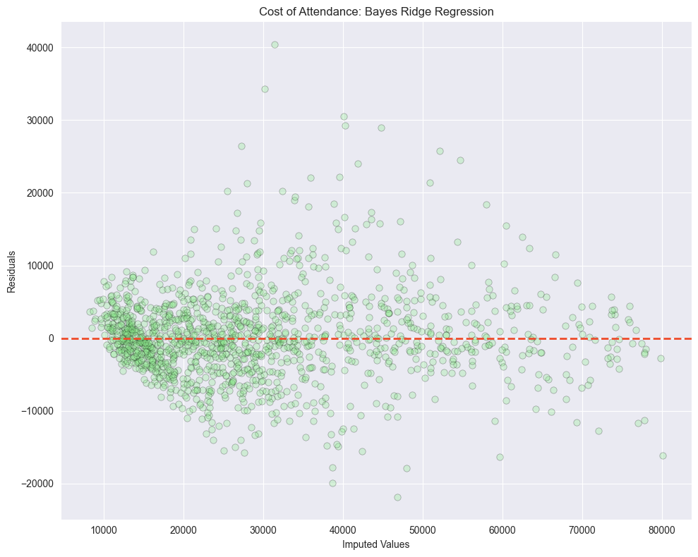
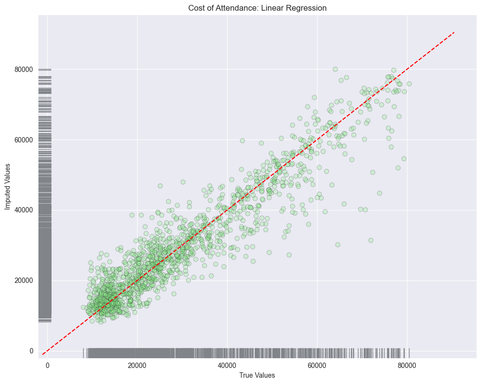
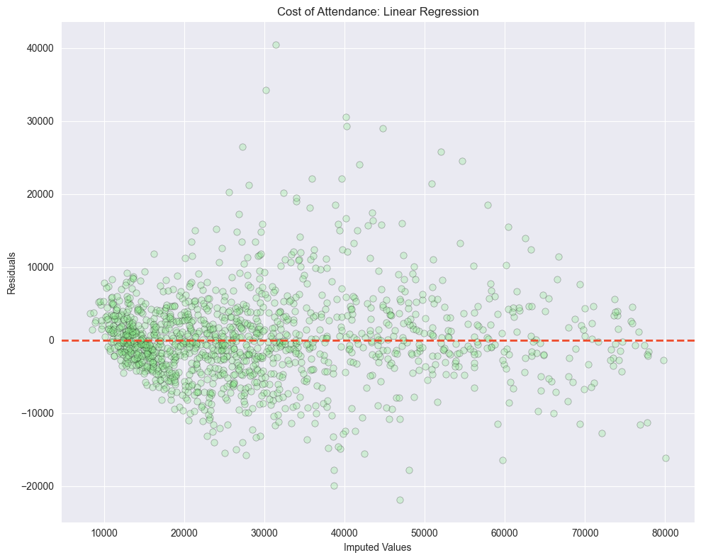
- Create concordance plots and residuals plot.
- Calculate Mean Absolute Error, Mean Squared Error, Root Mean Squared Error.
- Repeat with data transformations.
Basic algorithm
columns_to_impute = test_df.columns[1:]

# Get proporition of nulls
nulls = test_df.isna().sum()[1:] # excludes id column
proportion_of_nulls = round(nulls / len(test_df), 3)
proportion_list = list(proportion_of_nulls)

# Convert to dictionary
proportion_dict = dict(zip(columns_to_impute, proportion_list))

# Remove all nulls
test_df_clean = test_df[columns_to_impute].dropna(how="any").reset_index(drop=True)
test_df_to_impute = test_df_clean.copy()

for key in proportion_dict.keys():
    # get number of nulls
    num_null = int(len(test_df_to_impute) * proportion_dict[key])

    # randomly select indices
    null_indices = np.random.choice(test_df_to_impute.index, num_null, replace=False)

    # assign null vals to that column
    test_df_to_impute.loc[null_indices, key] = np.nan
Now, we will impute values with each model and save the results in a dataframe.
impute_techniques = {
    "bayesian_ridge_regression": IterativeImputer(random_state=45),
    "linear_regression": IterativeImputer(estimator=LinearRegression(), random_state=45),
    "random_forest": IterativeImputer(estimator=RandomForestRegressor(), random_state=45),
    "knn": KNNImputer()
    }

error_dicts = {name: {} for name in impute_techniques}
residuals_list = []

residuals_df = pd.DataFrame()

for name, imputer in impute_techniques.items():

    # Fit and transform the data once per imputer
    imputed_data = imputer.fit_transform(test_df_to_impute)
    imputed_df = pd.DataFrame(imputed_data, columns=columns_to_impute).round(2)

    for col in columns_to_impute:
        null_indices = test_df_to_impute[col].isnull()

        true_values = test_df_clean.loc[null_indices, col]
        predicted_values = imputed_df.loc[null_indices, col]

        mae = metrics.mean_absolute_error(true_values, predicted_values)
        mse = metrics.mean_squared_error(true_values, predicted_values)
        rmse = np.sqrt(mse)

        error_dicts[name][col] = [mae, mse, rmse]

        residuals = true_values.to_frame(name='true_value')
        residuals['predicted_value'] = predicted_values
        residuals = residuals.apply(pd.to_numeric)
        residuals['residuals'] = residuals['true_value'] - residuals['predicted_value']
        residuals['data_column'] = col
        residuals['impute_technique'] = name

        residuals_list.append(residuals)

residuals_df = pd.concat(residuals_list)

# sanity check print error dictionary for Bayesian Ridge Regression
print(error_dicts["bayesian_ridge_regression"])
Here are the results:
Bayesian Ridge Regression
Linear Regression
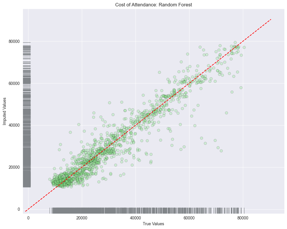
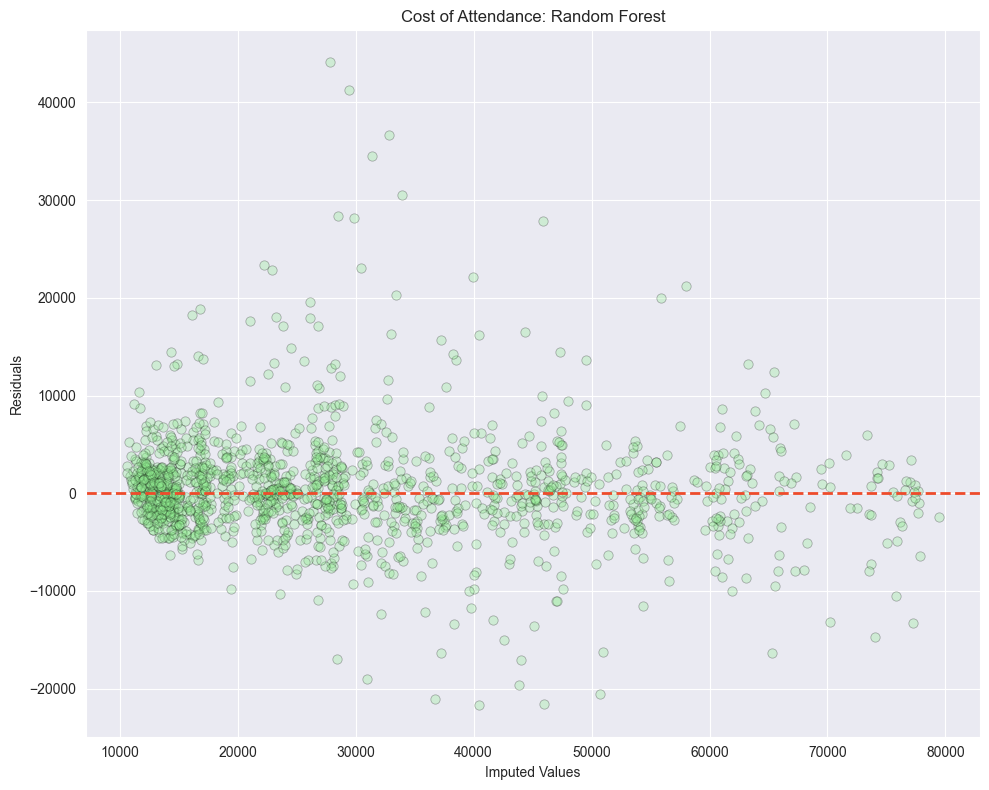
Random Forest
KNN
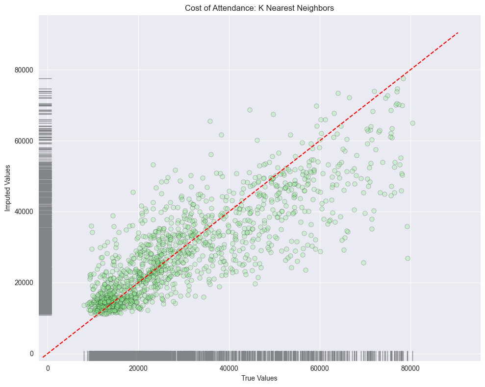
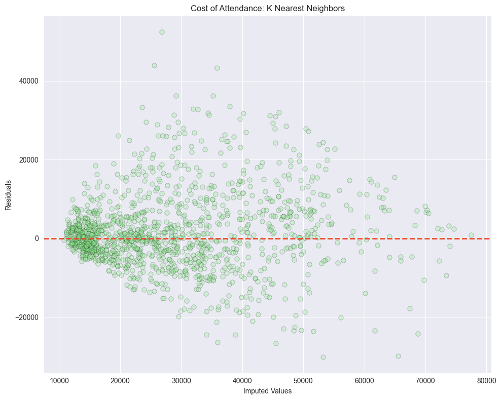
When we look at the error metrics we see that random forest did perform the best with the following results:
- MAE: $3,481.87
- MSE: 30,602,315.13
- RMSE: $5,531.94
Following random forest regression was bayes ridge regression:
- MAE: $4,292.5
- MSE: 37,296,221.96
- RMSE: $6,107.06
Looking at the residuals plots, we can see that all the algorithms struggled with the outliers at the higher ranges of data. And if we look at the distribution of all columns we see that none of the columns are normally distributed.
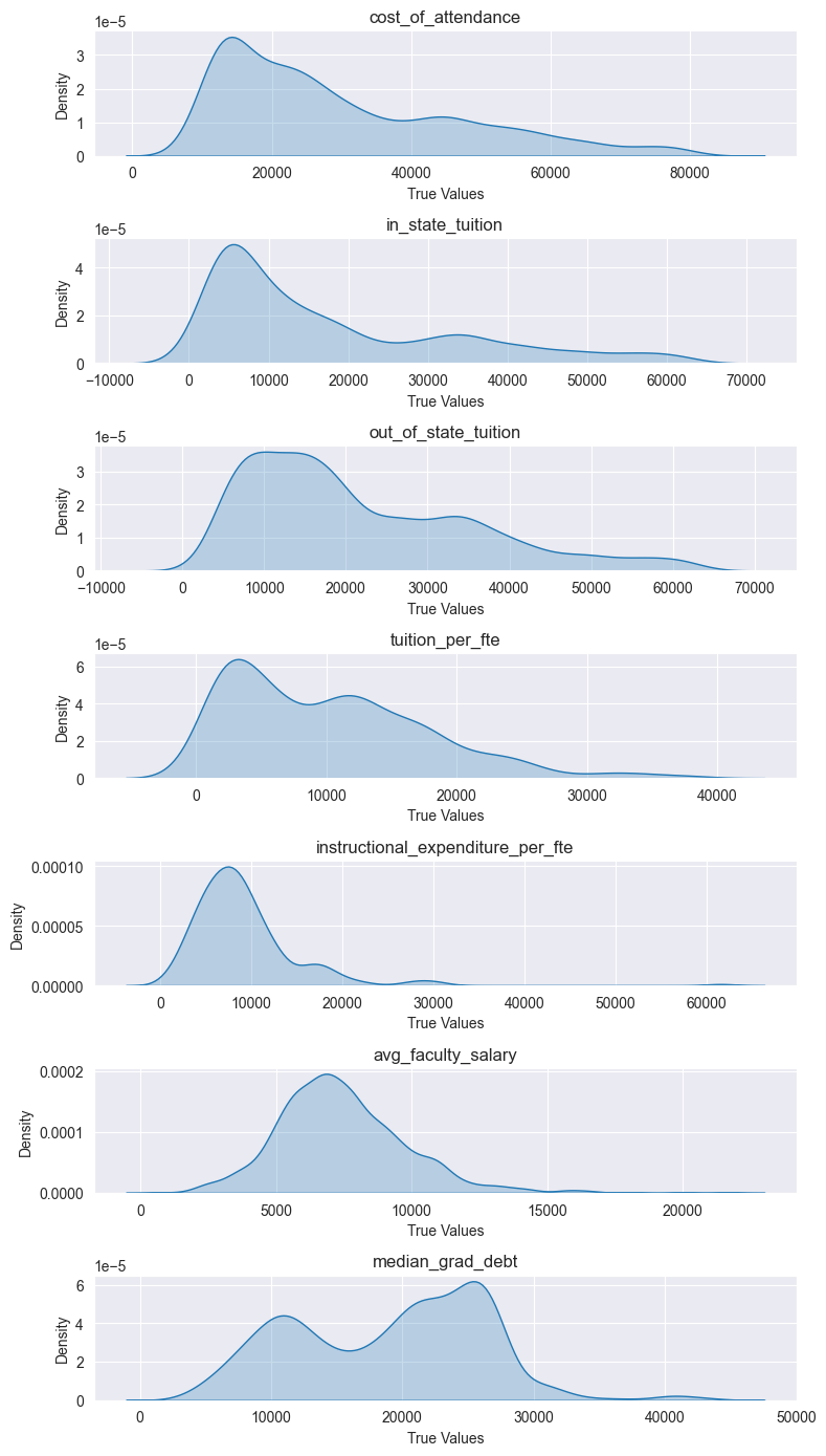
This will affect most algorithms that assume a Gaussian distribution. To mitigate this we can log transform the data.
Conclusion
I was going to do some feature engineering, like log transformating the variables to mitigate the skewness, and perform one-hot encoding to incorporate the regional categorical data into the models, but this post is a bit longer than I intended. If you enjoyed this post, stay tuned as I try an optimize these models as much as I can!
If you feel like this helped you out, feel free click the link below and support this post. Here’s my cat Vader for encouragement.
